LoRA — the low-rank trick, properly understood

LoRA (Low-Rank Adaptation) rests on one empirical discovery about fine-tuning itself:

When you fully fine-tune a model, each weight matrix W changes by some amount ΔW. The discovery: ΔW is almost always extremely redundant — the change, though spread across millions of numbers, has very few independent directions in it. In math terms, it has low rank.

Plain-language version of "rank": think of editing a photo. You could describe your edit as a list of changes to 12 million individual pixels. But if the edit was really "brightness +10, warmth +5, contrast +8," then three sliders fully describe those 12 million pixel changes. The rank is the number of independent sliders needed to describe the change. Fine-tuning changes, it turns out, are a few-slider kind of edit — makes sense, since Module 2 taught us fine-tuning mostly selects and amplifies existing behavior rather than installing new machinery.

The mechanism. Instead of learning the full-size ΔW (4096×4096 = 16.8M numbers per matrix), LoRA learns it as a product of two thin matrices: A (4096×r) and B (r×4096), where r — the rank — is tiny, like 16. The bypass output B·A·x gets added to the frozen path W·x:

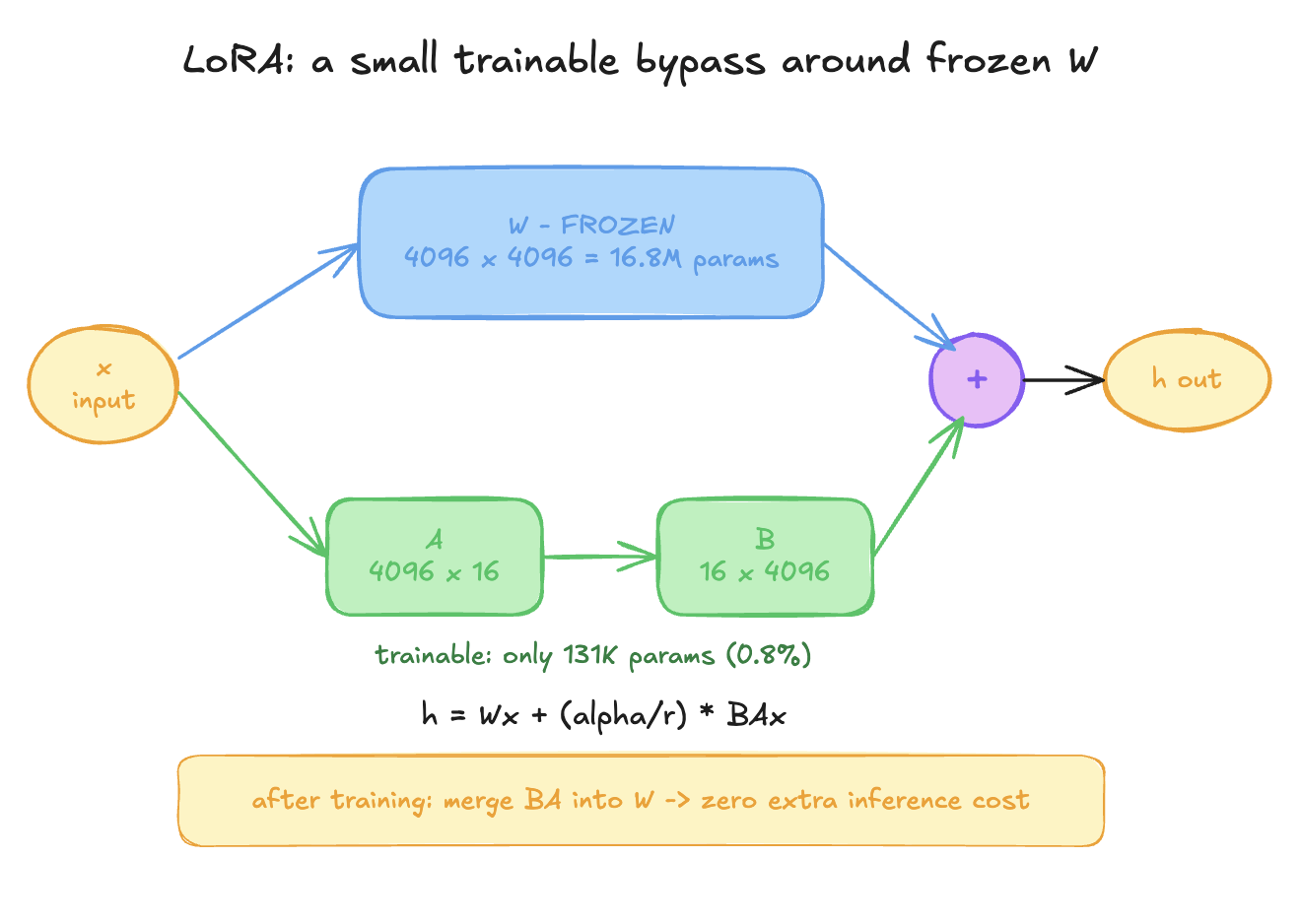
Count the savings in the diagram: the frozen matrix holds 16.8M parameters; the bypass holds 4096×16 + 16×4096 = 131K — under 1%. Apply this to every attention and MLP matrix across all 32 layers and a 7B model ends up with ~40M trainable parameters instead of 7B. Same steering wheel, 0.5% of the cost.

Three design details that reveal the elegance:

1. B starts at zero. A is initialized randomly, B as all zeros — so at step one, B·A·x = 0 and the bypass contributes nothing. Training begins from exactly the untouched base model and gradually grows a deviation. No random-initialization shock to a carefully-trained giant.
2. The α/r scaling (alpha in the formula) is just a volume knob on the bypass — how loudly the adaptation speaks over the base. Convention: set alpha = 2×r and forget about it.
3. The merge. After training, compute B·A once and add it into W permanently. The bypass vanishes; you're left with a single ordinary matrix. Zero extra inference latency — the property that killed classic adapters. Or don't merge, keep the adapter as a separate ~50 MB file, and hot-swap per Topic 22's wardrobe pattern. You choose per deployment.

The knobs you'll actually set (your first real hyperparameters, as promised in Lesson 2):

• r (rank): 8–64; start at 16. Higher = more capacity to change the model = more risk of overfitting your small dataset. Doubling r rarely doubles quality.
• target_modules: which matrices get bypasses. The original paper only did attention's Q and V; the modern default is all linear layers (attention + MLP — remember from Lesson 2 where the knowledge lives), which reliably helps.
• learning rate: ~1e-4 to 2e-4 — roughly 10× higher than full fine-tuning uses, because you're steering a tiny rudder, not the whole ship.

In code — this is the real thing, not pseudocode:

from peft import LoraConfig, get_peft_model
 
config = LoraConfig(r=16, lora_alpha=32, target_modules="all-linear",
                    lora_dropout=0.05, task_type="CAUSAL_LM")
model = get_peft_model(base_model, config)
model.print_trainable_parameters()
# trainable params: 40,370,176 || all params: 7,655,986,688 || trainable%: 0.53

That printout is the whole revolution in one line.

One advanced finding to carry with you (Biderman et al., 2024, neatly titled): "LoRA learns less and forgets less." With its low-rank bottleneck, LoRA has less capacity to absorb huge amounts of genuinely new material than full fine-tuning — but by the same token it damages the base model less, naturally resisting the catastrophic forgetting we battled throughout Module 2. For most fine-tuning jobs (form, style, task reliability — where the capability already exists in the base), this trade is a straight win: you didn't need the extra capacity, and you got the protection free. For continued-pretraining-scale knowledge injection (Topic 20), it's a real limitation — another reason that job uses full training.